TRIANGULATION_ORDER3 is a data directory which contains examples of triangulation data of order 3.
Defining a triangulation requires two files:
Other files that may be supplied include:
This is the simplest form of a triangulation. It is sometimes called a linear triangulation.
At the moment, no facility is provided for allowing the specification of constrained edges, or the existence of holes in the region, both of which are of some interest.
A node file can come from anywhere. In most cases, you generate this data by observation or the characteristics of a particular problem or set of data you are working on. In some cases, you start only with a region, and must fill the region with random points, or with well separated points.
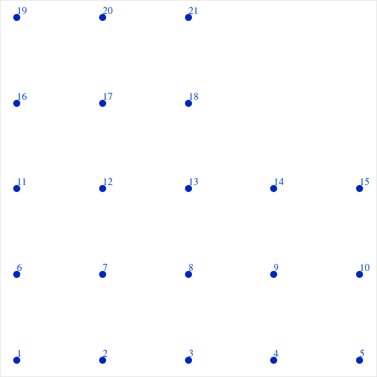
As a simple example, suppose we had the following set of points:
        19 20 21

        16 17 18

        11 12 13 14 15

         6  7  8  9 10

         1  2  3  4  5
then the node file might look like this:
        0.0  0.0
        1.0  0.0
        2.0  0.0
        3.0  0.0
        4.0  0.0
        0.0  1.0
        1.0  1.0
        2.0  1.0
        3.0  1.0
        4.0  1.0
        0.0  2.0
        1.0  2.0
        2.0  2.0
        3.0  2.0
        4.0  2.0
        0.0  3.0
        1.0  3.0
        2.0  3.0
        0.0  4.0
        1.0  4.0
        2.0  4.0
An element file describes how triangular elements are formed from the nodes. In an order 3 triangulation, each element is described by just 3 nodes. (An order 6 triangulation includes an extra node along the middle of each side). If you have nodes, but no triangulation of them, then there are programs available which can form a Delaunay triangulation of the nodes.
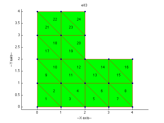
A possible order 3 triangulation of these nodes is:
        19-20-21
         |\ |\ |
         | \| \|
        16-17-18
         |\ |\ |
         | \| \|
        11-12-13-14-15
         |\ |\ |\ |\ |
         | \| \| \| \|
         6--7--8--9-10
         |\ |\ |\ |\ |
         | \| \| \| \|
         1--2--3--4--5
in which case the element file would look like this:
         1  2  6
         7  6  2
         2  3  7
         8  7  3
         3  4  8
         9  8  4
         4  5  9
        10  9  5
         6  7 11
        12 11  7
         7  8 12
        13 12  8
         8  9 13
        14 13  9
         9 10 14
        15 14 10
        11 12 16
        17 16 12
        12 13 17
        18 17 13
        16 17 19
        20 19 17
        17 18 20
        21 20 18
The elements could be listed in any order. The three nodes
of the element could be listed in any counterclockwise
order.
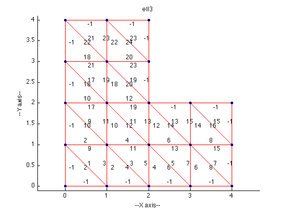
The element neighbor file lists the elements which are neighbors to a given element. The convention is that ELEMENT_NEIGHBOR(I,J) is the index of the element that is adjacent to the triangle on the side opposite ELEMENT_NODE(I,J). If there is no neighbor on that side then we set the entry to -1.
For the example problem, the neighbor file would look like:
 2  -1  -1
 1   3   9
 4   2  -1
 3   5  11
 6   4  -1
 5   7  13
 8   6  -1
 7  -1  15
10  -1   2
 9  11  17
12  10   4
11  13  19
14  12   6
13  15  -1
16  14   8
15  -1  -1
18  -1  10
17  19  21
20  18  12
19  -1  23
22  -1  18
21  23  -1
24  22  20
23  -1  -1
The boundary node file could list a 0 for each interior node, a 1 for each boundary node. This approach is convenient if inefficient, since it allows us to set aside space for the array immediately.
For the example problem, the boundarynode file would look like:
        1
        1
        1
        1
        1
        1
        0
        0
        0
        1
        1
        0
        1
        1
        1
        1
        0
        1
        1
        1
        1
An alternative format would simply list the indices of the boundary nodes:
         1
         2
         3
         4
         5
         6
        10
        11
        13
        14
        15
        16
        18
        19
        20
        21
and while this file lists the nodes in order, this is not essential.
We might wish to describe the boundary by listing the edges that form it. We would describe an edge as a pair of nodes. We will want to list these pairs in such a way that the boundary is traversed in counterclockwise order. Interior holes can also be handled this way, although then the curve is essentially traversed in clockwise order.
For the example problem, a boundary edge file might look like:
         1  2
         2  3
         3  4
         4  5
         5 10
        10 15
        15 14
        14 13
        13 18
        18 21
        21 20
        20 19
        19 16
        16 11
        11  6
         6  1
Although we have listed the edges in a way that traverses the entire
boundary consecutively, that is not of the highest importance.
The computer code and data files described and made available on this web page are distributed under the GNU LGPL license.
FEM2D, a data directory which contains examples of 2D FEM files, three text files that can be used to describe many finite element models;
FEM_BASIS_T3_DISPLAY a MATLAB program which displays a basis function associated with a 3-node triangle "T3" mesh.
MESH_BANDWIDTH a C++ program which returns the geometric bandwidth associated with a mesh of elements of any order and in a space of arbitrary dimension.
TRIANGULATE a C program which triangulates a (possibly nonconvex) polygon.
TRIANGULATION a C++ library which performs various operations on order 3 ("linear") or order 6 ("quadratic") triangulations.
TRIANGULATION_DISPLAY_OPENGL a C++ program which reads files defining a 2D triangulation and displays an image using OpenGL.
TRIANGULATION_ORDER3, a dataset directory of TRIANGULATION_ORDER3 files, a linear triangulation of a set of 2D points, using a pair of files to list the node coordinates and the 3 nodes that make up each triangle;
TRIANGULATION_ORDER4, a data directory which defines TRIANGULATION_ORDER4 files, a description of a triangulation of a set of 2D points, using a pair of files to list the node coordinates and the 4 nodes that make up each triangle (3 vertices and the centroid);
TRIANGULATION_ORDER6, a data directory which contains examples of TRIANGULATION_ORDER6 files, a description of a quadratic triangulation of a set of 2D points, using a pair of files to list the node coordinates and the 6 nodes that make up each triangle.
TRIANGULATION_ORIENT, a C++ program which ensures that the triangles in an order 3 or order 6 triangulation have positive orientation;
TRIANGULATION_PLOT is a C++ program which makes a PostScript image of a triangulation of points.
TRIANGULATION_QUALITY is a C++ program which computes quality measures of a triangulation.
ELL3 is an L-shaped region.
There are 21 nodes and 24 elements.
You can go up one level to the DATA page.